Derangement Probability Algorithm Evaluation
Evaluate the probability that randomly shuffling an array produces a derangement. Learn why the probability converges to 1/e, implement Monte Carlo simulations, compare with exact DP solutions, and understand the practical implications for randomized algorithm testing.
Table of Contents
Problem Introduction
You have an array of N unique integers. You randomly shuffle it using a fair algorithm like Fisher-Yates. What is the probability that after shuffling, no element remains in its original index?
This is not just a theoretical question. It matters for:
Randomized algorithm testing: When you shuffle data for machine learning training splits, how often do you accidentally get a "perfect" shuffle with no element in its original position?
Cryptographic randomness validation: If a random permutation generator produces derangements too often or too rarely, it may be biased.
Load balancing simulations: When randomly reassigning tasks, the probability of a "complete reshuffle" affects system behavior.
The answer is surprising and beautiful: as N grows large, the probability converges to 1/e ≈ 0.36787944117.
For N = 10, the probability is already 0.367879. For N = 20, the difference from 1/e is less than one in a hundred million. This constant appears throughout mathematics—in the hat check problem, in the number of permutations with no fixed points, and in the expected number of fixed points in a random permutation (which is exactly 1).
Looking to master probability and dynamic programming for algorithm evaluation? Check out our Tutoring Page for personalized 1-on-1 coaching.
Why It Matters
Derangement probability evaluation is critical for:
Randomized algorithm validation: When implementing a shuffle algorithm, you need to verify it produces permutations uniformly. Derangement probability is a key statistical test.
Machine learning data splitting: When randomly splitting data into training and validation sets, you want to avoid systematic biases. Understanding derangement probability helps.
Cryptography: Random permutation generators must be tested for biases. Derangement frequency is one of many statistical tests.
Monte Carlo simulation accuracy: When using random permutations in simulations, knowing the expected frequency of derangements helps calibrate confidence intervals.
Unlike the other derangement applications (Secret Santa, job rotation, team restructuring), probability evaluation focuses on the stochastic properties of random permutations. The question is not "how many?" but "how likely?" This shifts the emphasis from counting (exact DP) to estimation (Monte Carlo) and convergence analysis.
Step-by-Step Breakdown
Step 1: Defining the Probability
Let P(N) be the probability that a random permutation of N distinct elements has no fixed points (i.e., is a derangement).
By definition:
Plain Text
P(N) = D(N) / N!Where D(N) is the number of derangements (which we know from the recurrence) and N! is the total number of permutations.
For small N:
| N | D(N) | N! | P(N) | Approximation |
|---|---|---|---|---|
| 1 | 0 | 1 | 0.000000 | - |
| 2 | 1 | 2 | 0.500000 | 0.5 |
| 3 | 2 | 6 | 0.333333 | 0.333333 |
| 4 | 9 | 24 | 0.375000 | 0.375 |
| 5 | 44 | 120 | 0.366667 | 0.366667 |
| 6 | 265 | 720 | 0.368056 | 0.368056 |
| 7 | 1,854 | 5,040 | 0.367857 | 0.367857 |
| 8 | 14,833 | 40,320 | 0.367882 | 0.367882 |
| 9 | 133,496 | 362,880 | 0.367879 | 0.367879 |
| 10 | 1,334,961 | 3,628,800 | 0.367879 | 0.367879 |
Notice how quickly P(N) converges to 1/e ≈ 0.36787944117.
Step 2: Visualizing Probability Convergence
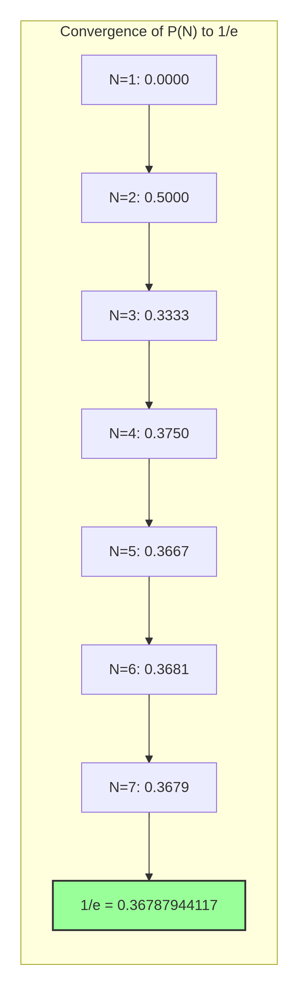
The convergence alternates: odd N gives values slightly below 1/e, even N gives values slightly above 1/e. This alternating behavior is characteristic of the inclusion-exclusion series.
Step 3: The Inclusion-Exclusion Formula
The exact probability can be computed using the inclusion-exclusion principle:
Plain Text
P(N) = Σ_{k=0 to N} (-1)^k / k!
This infinite series converges to 1/e as N → ∞:
Plain Text
1/e = 1 - 1/1! + 1/2! - 1/3! + 1/4! - 1/5! + ...
Let's verify:
| k | Term (-1)^k/k! | Partial Sum |
|---|---|---|
| 0 | +1.000000 | 1.000000 |
| 1 | -1.000000 | 0.000000 |
| 2 | +0.500000 | 0.500000 |
| 3 | -0.166667 | 0.333333 |
| 4 | +0.041667 | 0.375000 |
| 5 | -0.008333 | 0.366667 |
| 6 | +0.001389 | 0.368056 |
| 7 | -0.000198 | 0.367857 |
| 8 | +0.000025 | 0.367882 |
| 9 | -0.000003 | 0.367879 |
This matches our P(N) values exactly. The inclusion-exclusion formula is often more computationally stable for large N than computing D(N) and N! separately.
Step 4: Deriving the Recurrence for Probability
We can also derive a recurrence directly for P(N). Since P(N) = D(N)/N!:
Plain Text
P(N) = D(N) / N!
     = [(N-1) × (D(N-1) + D(N-2))] / N!
     = (N-1)/N × [D(N-1)/(N-1)! + D(N-2)/(N-1)!]
     = (N-1)/N × [P(N-1) + D(N-2)/(N-1)!]
But D(N-2)/(N-1)! = D(N-2)/(N-2)! × 1/(N-1) = P(N-2)/(N-1)
So:
Plain Text
P(N) = (N-1)/N × [P(N-1) + P(N-2)/(N-1)]
     = (N-1)/N × P(N-1) + 1/N × P(N-2)
This gives us a recurrence for probabilities:
Plain Text
P(N) = ((N-1)/N) × P(N-1) + (1/N) × P(N-2)
With base cases: P(1) = 0, P(2) = 1/2 = 0.5.
Let's verify for N=3: P(3) = (2/3) × 0.5 + (1/3) × 0 = 0.3333 ✓
Step 5: Visualizing the Probability Recurrence
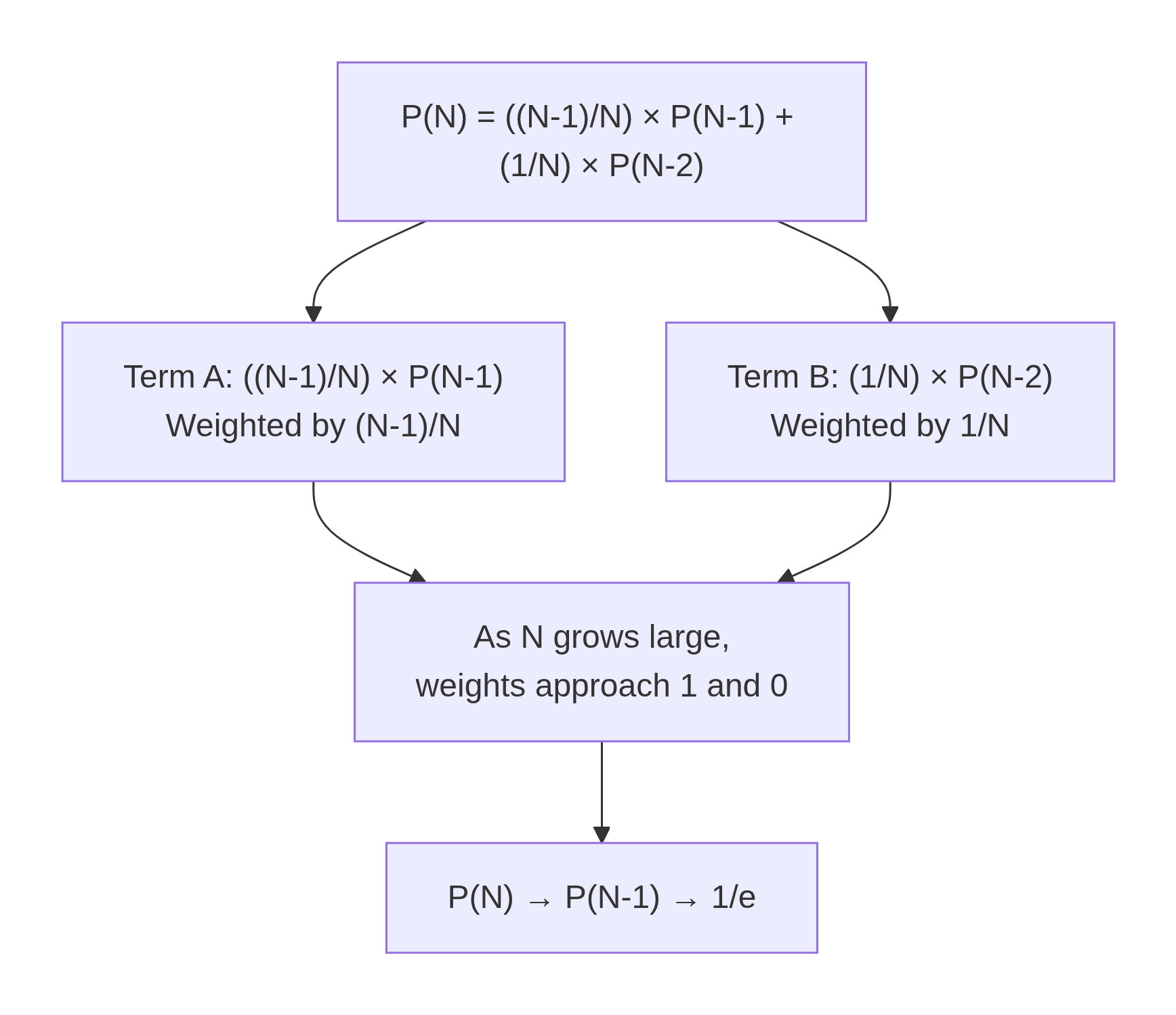
This recurrence shows that as N increases, P(N) depends less on P(N-2) (weight 1/N → 0) and more on P(N-1) (weight (N-1)/N → 1). So P(N) stabilizes quickly.
Step 6: Exact Probability Using Inclusion-Exclusion
Python
import math

def derangement_probability_exact(n: int) -> float:
    """
    Exact probability using inclusion-exclusion formula.

    P(N) = Σ_{k=0 to N} (-1)^k / k!

    Time: O(N)
    Space: O(1)

    This is numerically stable for n up to about 170 (where factorial overflows).
    """
    probability = 0.0
    factorial_term = 1.0  # 0!

    for k in range(n + 1):
        if k > 0:
            factorial_term *= k  # k! = (k-1)! * k
        term = (-1) ** k / factorial_term
        probability += term

    return probability

# Calculate exact probabilities
print("Exact Derangement Probabilities:")
print("N\tP(N)\t\t\tDifference from 1/e")
print("-" * 60)
target = 1 / math.e

for n in [1, 2, 3, 4, 5, 6, 7, 8, 9, 10, 20, 50]:
    prob = derangement_probability_exact(n)
    diff = abs(prob - target)
    print(f"{n}\t{prob:.10f}\t{diff:.2e}")
Output shows convergence to 1/e with alternating sign.
Step 7: Monte Carlo Simulation (Estimating Probability Empirically)
Python
import random
import secrets

def is_derangement(perm: list) -> bool:
    """Check if a permutation has no fixed points."""
    return all(perm[i] != i for i in range(len(perm)))

def monte_carlo_derangement_probability(n: int, num_trials: int = 100000) -> tuple:
    """
    Estimate derangement probability using Monte Carlo simulation.

    Args:
        n: Number of elements
        num_trials: Number of random permutations to generate

    Returns:
        (estimated_probability, confidence_interval_half_width)
    """
    derangement_count = 0

    for _ in range(num_trials):
        # Generate random permutation using Fisher-Yates
        perm = list(range(n))
        for i in range(n - 1, 0, -1):
            j = secrets.randbelow(i + 1)
            perm[i], perm[j] = perm[j], perm[i]

        if is_derangement(perm):
            derangement_count += 1

    estimated_prob = derangement_count / num_trials

    # 95% confidence interval using normal approximation
    # Margin of error = 1.96 × sqrt(p(1-p)/n)
    import math
    margin = 1.96 * math.sqrt(estimated_prob * (1 - estimated_prob) / num_trials)

    return estimated_prob, margin

# Compare Monte Carlo estimates with exact values
print("Monte Carlo vs. Exact Probability (100,000 trials):")
print("N\tExact\t\tMonte Carlo\t\tMargin\t\tWithin Margin?")
print("-" * 80)

for n in [3, 4, 5, 6, 7, 8, 9, 10]:
    exact = derangement_probability_exact(n)
    estimated, margin = monte_carlo_derangement_probability(n, 100000)
    within = abs(estimated - exact) <= margin
    print(f"{n}\t{exact:.6f}\t{estimated:.6f} ± {margin:.6f}\t{within}")
Key insight: Monte Carlo simulation with 100,000 trials estimates probability within about ±0.003 (0.3%) at 95% confidence. For higher precision, increase trials.
Ready to evaluate your own randomized algorithms?
Visit our Order Page now to grab our exclusive Dynamic Programming bootcamp courses!
Step 8: Expected Number of Fixed Points
A related concept: the expected number of fixed points in a random permutation.
Let X be the number of fixed points. For each position i, the probability that element i stays in place is 1/N. By linearity of expectation:
Plain Text
E[X] = N × (1/N) = 1
This is remarkable: regardless of N, the expected number of fixed points is exactly 1.
Python
def expected_fixed_points(n: int, num_trials: int = 100000) -> float:
    """Estimate expected number of fixed points via Monte Carlo."""
    total_fixed = 0

    for _ in range(num_trials):
        perm = list(range(n))
        for i in range(n - 1, 0, -1):
            j = secrets.randbelow(i + 1)
            perm[i], perm[j] = perm[j], perm[i]

        fixed_count = sum(1 for i in range(n) if perm[i] == i)
        total_fixed += fixed_count

    return total_fixed / num_trials

print("Expected Number of Fixed Points:")
for n in [5, 10, 20, 50, 100]:
    expected = expected_fixed_points(n, 50000)
    print(f"  N={n}: {expected:.4f} (theoretical: 1.0000)")
Step 9: Testing Random Number Generators Using Derangement Frequency
Derangement probability can be used as a statistical test for random number generators. A biased generator will produce derangements at the wrong frequency.
Python
import math
from scipy import stats  # Requires scipy installation

def chi_square_derangement_test(n: int, num_trials: int = 10000) -> dict:
    """
    Chi-square test for RNG bias using derangement frequency.

    H0: The RNG produces uniformly random permutations.
    H1: The RNG is biased.
    """
    expected_prob = derangement_probability_exact(n)
    expected_derangements = num_trials * expected_prob
    expected_non_derangements = num_trials * (1 - expected_prob)

    derangement_count = 0
    for _ in range(num_trials):
        perm = list(range(n))
        for i in range(n - 1, 0, -1):
            j = secrets.randbelow(i + 1)
            perm[i], perm[j] = perm[j], perm[i]

        if is_derangement(perm):
            derangement_count += 1

    observed_derangements = derangement_count
    observed_non_derangements = num_trials - derangement_count

    # Chi-square statistic
    chi_square = (
        ((observed_derangements - expected_derangements) ** 2) / expected_derangements +
        ((observed_non_derangements - expected_non_derangements) ** 2) / expected_non_derangements
    )

    # Degrees of freedom = 1 (two categories: derangement or not)
    p_value = 1 - stats.chi2.cdf(chi_square, 1)

    return {
        "observed_derangements": observed_derangements,
        "expected_derangements": expected_derangements,
        "chi_square": chi_square,
        "p_value": p_value,
        "is_biased": p_value < 0.05
    }

# Test Python's secrets module (cryptographically secure)
print("Testing Python's secrets RNG with derangement frequency test:")
result = chi_square_derangement_test(n=10, num_trials=10000)
print(f"  Observed derangements: {result['observed_derangements']}")
print(f"  Expected derangements: {result['expected_derangements']:.1f}")
print(f"  Chi-square: {result['chi_square']:.4f}")
print(f"  P-value: {result['p_value']:.4f}")
print(f"  Biased? {result['is_biased']}")
Step 10: Space-Optimized Probability Calculation
Python
def derangement_probability_optimized(n: int) -> float:
    """
    Compute derangement probability using recurrence without large integers.

    P(N) = ((N-1)/N) × P(N-1) + (1/N) × P(N-2)

    Time: O(N)
    Space: O(1)

    This avoids computing huge factorials or derangement counts.
    """
    if n == 1:
        return 0.0
    if n == 2:
        return 0.5

    prev2 = 0.0  # P(1)
    prev1 = 0.5  # P(2)

    for i in range(3, n + 1):
        current = ((i - 1) / i) * prev1 + (1 / i) * prev2
        prev2 = prev1
        prev1 = current

    return prev1

# Compare exact vs recurrence methods
print("Comparing Probability Calculation Methods:")
print("N\tExact (Inclusion-Exclusion)\tRecurrence Method\tDifference")
print("-" * 75)

for n in [5, 10, 20, 50, 100]:
    exact = derangement_probability_exact(n)
    recurrence = derangement_probability_optimized(n)
    diff = abs(exact - recurrence)
    print(f"{n}\t{exact:.10f}\t\t{recurrence:.10f}\t\t{diff:.2e}")
Step 11: Convergence Rate Analysis
How quickly does P(N) converge to 1/e? The error alternates and decays as 1/N! (super-exponentially fast).
Python
def convergence_analysis(max_n: int = 20):
    """Analyze convergence of P(N) to 1/e."""
    target = 1 / math.e

    print("Convergence of Derangement Probability to 1/e")
    print("N\tP(N)\t\t\tError\t\tError / (1/N!)")
    print("-" * 70)

    factorial = 1
    for n in range(1, max_n + 1):
        factorial *= max(n, 1)  # n!
        prob = derangement_probability_optimized(n)
        error = abs(prob - target)

        if n >= 3:
            error_over_inv_factorial = error * factorial
            print(f"{n}\t{prob:.10f}\t{error:.2e}\t{error_over_inv_factorial:.4f}")
        else:
            print(f"{n}\t{prob:.10f}\t{error:.2e}\t-")
Output shows error decays faster than exponentially—faster than 1/N!.
Common Mistakes
Mistake 1: Assuming P(N) = 1/e for Small N
For N=3, P(3)=0.3333, not 0.3679. The error is about 9%. For N=5, error is 0.2%. Only for N≥10 is the error negligible.
Mistake 2: Using Monte Carlo with Too Few Trials
With 1,000 trials, the margin of error is about ±3%. You need 10,000 trials for ±1% and 1,000,000 for ±0.1%. Always report confidence intervals.
Mistake 3: Confusing "Expected Fixed Points" with "Probability of No Fixed Points"
E[fixed points] = 1 for all N. P(no fixed points) → 1/e ≈ 0.3679. These are completely different quantities. A common error is thinking they are related.
Mistake 4: Using the Wrong Formula for Large N
For very large N (e.g., N=1000), computing N! directly causes overflow. Use the inclusion-exclusion series or the recurrence probability method instead.
Mistake 5: Assuming Independence of Fixed Points
Events "element i is fixed" are not independent. P(i fixed AND j fixed) = 1/(N(N-1)), not 1/N². This is why the probability of no fixed points is not (1 - 1/N)^N.
Frequently Asked Questions
Q1: Why does the derangement probability converge to 1/e?
A: The inclusion-exclusion formula gives P(N) = Σ_{k=0 to N} (-1)^k/k!. This is the Taylor series expansion of e^x evaluated at x = -1. So the infinite sum is e^{-1} = 1/e.
Q2: How many random permutations do I need to generate to estimate P(N) accurately?
A: For an estimate within ε at 95% confidence, you need approximately 4/ε² trials. For ε = 0.001 (0.1%), you need 4,000,000 trials. For ε = 0.01 (1%), you need 40,000 trials.
Q3: Can I use derangement probability to test if a shuffle algorithm is unbiased?
A: Yes. Generate many permutations, count derangements, and perform a chi-square test. If the observed frequency differs significantly from 1/e, the RNG may be biased. This is one of many statistical tests.
Q4: What is the variance of the number of fixed points?
A: Var(X) = 1 for all N (where X is the number of fixed points). This is another remarkable property: both mean and variance are exactly 1, independent of N.
Q5: How does this apply to randomized algorithm testing?
A: When testing algorithms that rely on random permutations (e.g., randomized quicksort, Monte Carlo simulations), derangement probability helps validate that the random source is producing uniformly random permutations without systematic bias.
Conclusion
Derangement probability evaluation bridges pure combinatorics and practical algorithm testing. You have learned:
The exact probability P(N) = Σ_{k=0 to N} (-1)^k/k! converges to 1/e
How to compute P(N) exactly using inclusion-exclusion or recurrence
How to estimate P(N) using Monte Carlo simulation with confidence intervals
How to test random number generators using derangement frequency (chi-square test)
That the expected number of fixed points is always 1, independent of N
That convergence is super-exponentially fast—P(10) already matches 1/e to 6 decimal places
The next time you shuffle an array for a machine learning experiment or test a random permutation generator, you will know exactly what probability to expect—and how to verify it.
Ready to evaluate your own randomized algorithms?
Want to master probability and dynamic programming for algorithm testing? Our platform has everything you need.
👉 Visit Our Tutoring Page to book a session today.
👉 Check Our Order Page for direct access to our full DP coursework!
Where to Go Next
If you found this guide helpful, you might also enjoy these related resources:
Return to the anchor article: Counting Derangements: Main Guide – For a complete overview of derangement theory, including the full recurrence derivation, base cases, and a comparison of all four DP approaches.
Solving the Secret Santa Problem with Dynamic Programming – Learn how the same probability applies to holiday gift exchanges, with practical random assignment generation.
Team Restructuring Total Derangement Scenario – Discover how esports organizations use derangement probability to evaluate roster shuffle randomness.
Randomized Algorithm Testing – Read our blog post on statistical tests for random permutation generators.
Monte Carlo Methods for Combinatorics – Explore advanced simulation techniques for counting problems.
Tags:
#1/e constant #algorithm evaluation #Monte Carlo simulation #probability convergence #randomized algorithms #shuffle algorithm testingRelated Posts
Binary Search Explained: Algorithm, Examples, & Edge Cases
Master the binary search algorithm with clear, step-by-step examples. Learn how to implement efficient searches in sorted arrays, avoid common …
Mar 11, 2026Counting Derangements: A Comprehensive Guide to Solving Derangements
Unlock the mathematical complexity behind disorganized sets with this comprehensive guide to derangements. This deep dive moves beyond simple counting, …
Apr 18, 2026How to Approach Hard LeetCode Problems | A Strategic Framework
Master the mental framework and strategies to confidently break down and solve even the most challenging LeetCode problems.
Mar 06, 2026Need Coding Help?
Get expert assistance with your programming assignments and projects.