General Gift Exchange Combinatorics

Problem Introduction

Imagine a large corporation with N departments: HR, IT, Sales, Marketing, Finance, Operations, Legal, and R&D. Each year, the company holds a gift exchange—but not between individuals. Departments give gifts to other departments. The only rule? A department cannot give a gift to itself. HR cannot gift HR. IT cannot gift IT.

This shifts the classic Secret Santa problem from individuals to nodes in an organizational chart. The mathematics remain the same—derangements—but the interpretation changes. Instead of people drawing names, we have departments trading value, information, or resources.

Now expand this idea further. What if each department must also receive exactly one gift? That creates a perfect matching—a permutation of N departments with no fixed points. In graph theory terms, we are counting the number of derangements on a complete directed graph where self-loops are forbidden.

For N = 5 departments, how many valid gift-exchange mappings exist? The answer is 44. For N = 10 departments, it is 1,334,961. These numbers scale super-exponentially, and understanding them is crucial for designing fair, unpredictable, and secure exchange systems at the organizational level.

Why It Matters

General gift exchange combinatorics extends far beyond holiday parties. This derangement model applies to:

• Macroeconomics and supply chain inter-trading: When N companies form a trading network where no company trades with itself, the number of possible trading configurations is a derangement count. This helps economists model market diversity and prevent monopolistic self-dealing.

• Inter-departmental auditing: Financial controls often require that no department audits itself. The number of possible audit rotation schedules is a derangement problem.

• Cryptographic key distribution: In some key-exchange protocols, nodes must establish pairwise connections without self-mapping. Derangements ensure no node is paired with itself.

• Load balancing in distributed systems: When N servers forward requests to each other, derangements prevent a server from sending traffic to itself (which would create a loop).

Unlike the individual-focused Secret Santa, the general gift exchange operates at the level of aggregate entities. The constraints are identical—no fixed points—but the stakes are higher. A department accidentally gifting itself might mean a budget misallocation or an internal audit failure. A company trading with itself in a supply chain model breaks the assumption of market diversity.

Looking to master dynamic programming for real-world systems? Check out our  Tutoring Page  for personalized 1-on-1 coaching.

Step-by-Step Breakdown

Step 1: Restating as a Directed Graph Problem

Let the N departments be nodes in a directed graph. A valid gift exchange is a permutation (a set of directed edges) such that:

• Every department has exactly one outgoing edge (gives one gift)

• Every department has exactly one incoming edge (receives one gift)

• No department has an edge pointing to itself (no self-gifting)

This is a derangement of N items. The number of such permutations is !N (subfactorial N).

Step 2: Visualizing with a Multi-Department Flow

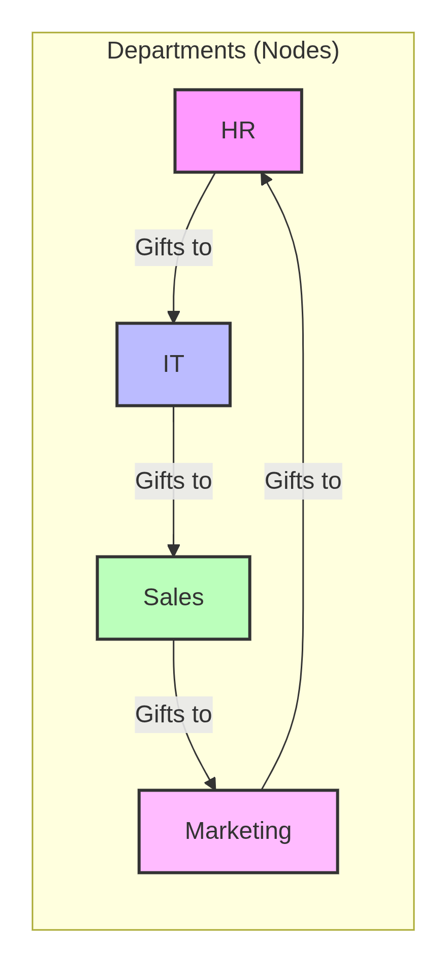
In this diagram, we have a 4-cycle: HR → IT → Sales → Marketing → HR. No department gives to itself. This is one valid gift exchange configuration. Other valid configurations might include two 2-cycles (HR↔IT, Sales↔Marketing) or a 3-cycle plus a fixed-point-free arrangement of the remaining department (which for N=4 is impossible since a 3-cycle leaves one department that would have to self-gift).

Step 3: Building Intuition with Small N

Let G(N) be the number of valid department gift exchanges.

N = 1 (single department): The only possible gift is to itself. This violates the rule. G(1) = 0.

N = 2 (two departments: HR and IT): Valid arrangements:

• HR → IT, IT → HR (swap)

• That's it. G(2) = 1.

N = 3 (three departments): Let's list all 6 permutations of [HR, IT, Sales] and check for self-gifts:

• [HR, IT, Sales] → all self-gift (invalid)

• [HR, Sales, IT] → HR self-gifts (invalid)

• [IT, HR, Sales] → Sales self-gifts (invalid)

• [IT, Sales, HR] → no self-gifts (valid)

• [Sales, HR, IT] → no self-gifts (valid)

• [Sales, IT, HR] → IT self-gifts (invalid)

G(3) = 2.

N = 4: The number jumps to 9. Notice the pattern: 0, 1, 2, 9, 44, 265, 1854, 14833...

Step 4: Deriving the Recurrence Relation (Department Perspective)

Let G(N) be the number of valid gift exchanges for N departments.

Step A: Where does Department 1 send its gift?
Department 1 cannot send to itself. So it sends to Department k, where k ∈ {2, 3, ..., N}. That's (N - 1) possibilities.

Step B: Analyze Department k's gift recipient.
Now consider where Department k sends its gift. Two scenarios:

Scenario 1: Department k sends its gift to Department 1

• Department 1 → Department k, Department k → Department 1

• These two departments have swapped gifts

• The remaining (N - 2) departments must form a valid gift exchange among themselves

• Number of ways: G(N - 2)

Scenario 2: Department k sends its gift to someone else (not Department 1)

• Department 1 → Department k

• Department k cannot send to Department 1 (by this scenario) and also cannot send to itself (original position)

• This is equivalent to finding a valid gift exchange for the remaining (N - 1) departments, where Department k is now forbidden from sending to Department 1

• Number of ways: G(N - 1)

Step C: Combine the cases
For each of the (N - 1) choices for Department 1's recipient:

G(N) = (N - 1) × [G(N - 1) + G(N - 2)]

Base cases: G(1) = 0, G(2) = 1.

Check: G(3) = 2 × (G(2) + G(1)) = 2 × (1 + 0) = 2 ✓
G(4) = 3 × (G(3) + G(2)) = 3 × (2 + 1) = 9 ✓

Step 5: Visualizing the Recurrence with Department Swaps

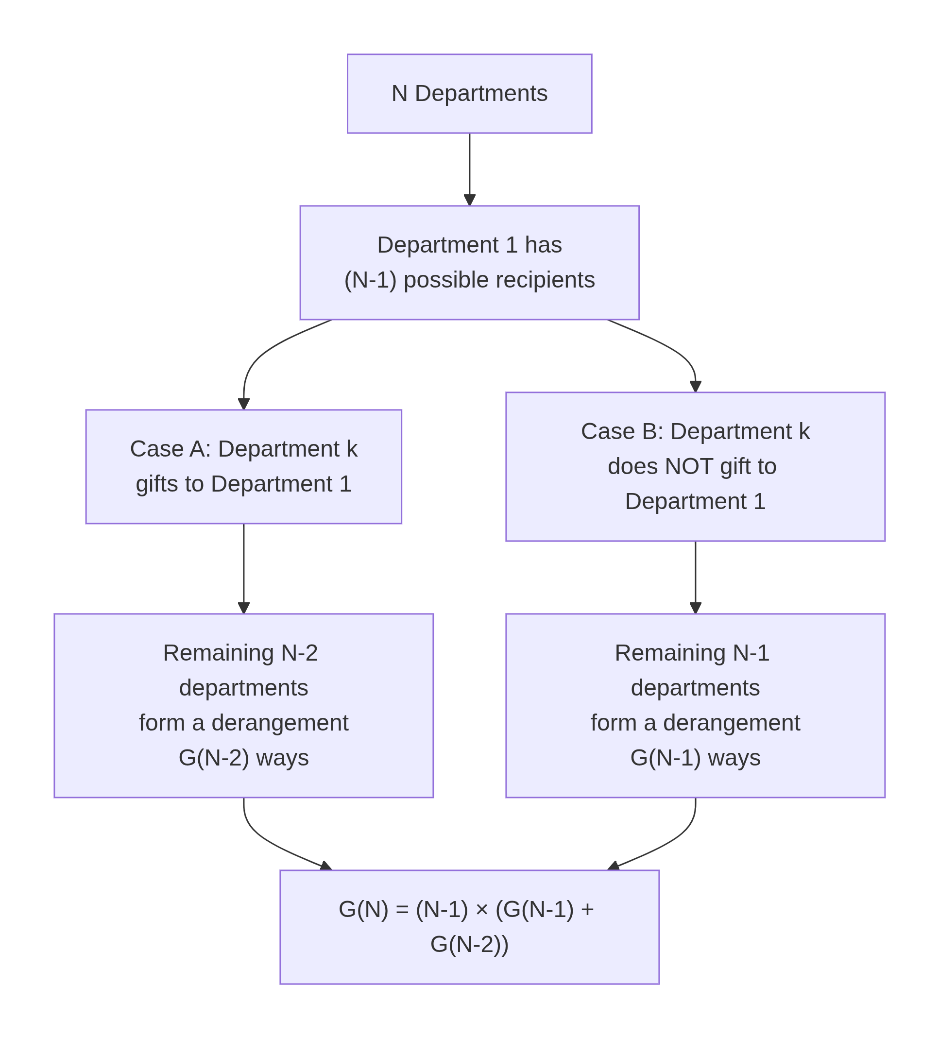
This flowchart shows the branching logic from the perspective of a macro-level entity (department) rather than an individual person. 

The key insight is that the structure is identical to individual derangements, but the interpretation—organizational units trading value—opens new applications.

Step 6: Naive Recursive Implementation

def gift_exchange_recursive(departments: int) -> int:
    """
    Naive recursive solution for department gift exchanges.
    
    Time: O(2^N) - Exponential, impractical for N > 30
    Space: O(N) - Recursion stack depth
    
    This directly implements G(N) = (N-1) * (G(N-1) + G(N-2)).
    """
    if departments == 1:
        return 0  # One department cannot avoid self-gifting
    if departments == 2:
        return 1  # Only a swap between two departments
    
    return (departments - 1) * (
        gift_exchange_recursive(departments - 1) + 
        gift_exchange_recursive(departments - 2)
    )

# Example for a small company with 5 departments
print(f"G(5) = {gift_exchange_recursive(5)}")  # 44

Why recursion fails for real companies: A typical corporation might have 20-30 departments. Computing G(30) recursively would require over 2^30 ≈ 1 billion function calls. On a standard laptop, that would take hours or days.

Step 7: Top-Down DP with Memoization (Department-Level Caching)

def gift_exchange_top_down(departments: int, memo: dict = None) -> int:
    """
    Top-down dynamic programming with memoization.
    
    Time: O(N) - Each N computed once
    Space: O(N) - Memo dictionary + recursion stack
    
    This approach caches results for each department count,
    making large N (e.g., 1000) computationally feasible.
    """
    if memo is None:
        memo = {}
    
    if departments == 1:
        return 0
    if departments == 2:
        return 1
    if departments in memo:
        return memo[departments]
    
    memo[departments] = (departments - 1) * (
        gift_exchange_top_down(departments - 1, memo) + 
        gift_exchange_top_down(departments - 2, memo)
    )
    return memo[departments]

# Example for a large corporate structure
print(f"G(20) = {gift_exchange_top_down(20):,}")
# Output: 895,014,631,192,902,121 (approximately 8.95 × 10^17)

Insight for system designers: The memoization dictionary acts like a cache for computed derangement values. If your organization frequently needs G(N) for various N (e.g., for different teams or subsidiaries), caching provides massive speedups.

Ready to optimize your department rotation systems?

Visit our Order Page now to grab our exclusive Dynamic Programming bootcamp courses!

Step 8: Bottom-Up DP with Tabulation (Iterative Construction)

def gift_exchange_bottom_up(departments: int) -> int:
    """
    Bottom-up dynamic programming using tabulation.
    
    Time: O(N)
    Space: O(N) - Full DP array
    
    This approach is useful when you need all intermediate values
    for analysis or visualization (e.g., plotting growth rates).
    """
    if departments == 1:
        return 0
    if departments == 2:
        return 1
    
    # dp[i] = number of valid gift exchanges for i departments
    dp = [0] * (departments + 1)
    dp[1] = 0
    dp[2] = 1
    
    for i in range(3, departments + 1):
        dp[i] = (i - 1) * (dp[i - 1] + dp[i - 2])
    
    return dp[departments]

# Analyze growth for department counts
def analyze_gift_exchange_growth(max_depts: int = 15):
    """Show how G(N) grows with N and compare to N! (total permutations)."""
    print("Depts\tG(N)\t\t\tN!\t\t\tRatio G(N)/N!")
    print("-" * 70)
    from math import factorial
    for n in range(1, max_depts + 1):
        g = gift_exchange_bottom_up(n)
        fact = factorial(n)
        ratio = g / fact if fact > 0 else 0
        print(f"{n}\t{g:>20,}\t{fact:>20,}\t{ratio:.6f}")

analyze_gift_exchange_growth()

Output snippet:

Depts   G(N)                    N!                      Ratio G(N)/N!
1                       0                       1       0.000000
2                       1                       2       0.500000
3                       2                       6       0.333333
4                       9                      24       0.375000
5                      44                     120       0.366667
6                     265                     720       0.368056
7                   1,854                   5,040       0.367857
8                  14,833                  40,320       0.367882
9                 133,496                 362,880       0.367879
10              1,334,961               3,628,800       0.367879

Notice the ratio converges to 1/e ≈ 0.367879. This means that for large department counts, approximately 36.79% of all possible gift-exchange mappings are valid (no self-gifting).

Step 9: Space-Optimized Solution for Supply Chain Systems

def gift_exchange_optimized(departments: int) -> int:
    """
    Space-optimized bottom-up solution.
    
    Time: O(N)
    Space: O(1) - Only two variables
    
    This is the optimal solution for implementing in production
    systems where memory efficiency matters (e.g., embedded devices,
    high-frequency trading systems, or large-scale simulations).
    """
    if departments == 1:
        return 0
    if departments == 2:
        return 1
    
    # prev2 = G(i-2), prev1 = G(i-1)
    prev2 = 0  # G(1)
    prev1 = 1  # G(2)
    
    for i in range(3, departments + 1):
        current = (i - 1) * (prev1 + prev2)
        prev2 = prev1
        prev1 = current
    
    return prev1

# Real-world example: How many valid trading configurations for 50 companies?
# G(50) has approximately 63 digits. Python handles it easily.
g_50 = gift_exchange_optimized(50)
print(f"G(50) = {g_50}")
print(f"Number of digits: {len(str(g_50))}")
# Output: 63 digits, roughly 2.96 × 10^62

Why space optimization matters in supply chain models: If you are simulating trillions of possible inter-company trading networks, storing a full DP array for N=10,000 would require ~80 KB (10,000 × 8 bytes). That's fine. But if you are running on an embedded device or need to compute G(N) for millions of different N values in a loop, O(1) space becomes critical.

Step 10: From Departments to Weighted Graphs (Advanced Extension)

In real supply chains, not all department-to-department gifts are equally likely or equally valuable. Some departments might prefer to trade with certain others due to logistics, cost, or strategic alignment.

This leads to the concept of weighted derangements: counting derangements where each mapping has a weight (probability, cost, or value). The total number of weighted derangements is the permanent of a matrix with zeros on the diagonal—a #P-complete problem (computationally intractable for large N).

For small N (≤ 20), you can compute weighted derangements using the inclusion-exclusion formula with weight products. For larger N, you use Monte Carlo Markov Chain (MCMC) sampling.

import random

def sample_weighted_derangement(weights: list, n_samples: int = 10000) -> float:
    """
    Approximate the total weight of all derangements using Monte Carlo sampling.
    
    Args:
        weights: N x N matrix where weights[i][j] = weight of department i giving to j
        n_samples: Number of random permutations to sample
        
    Returns:
        Estimated total weight across all derangements
    """
    N = len(weights)
    total_weight = 0
    valid_samples = 0
    
    for _ in range(n_samples):
        # Generate a random permutation
        perm = list(range(N))
        random.shuffle(perm)
        
        # Check if it's a derangement (no fixed points)
        if all(perm[i] != i for i in range(N)):
            # Compute product of weights for this permutation
            weight_product = 1
            for i in range(N):
                weight_product *= weights[i][perm[i]]
            total_weight += weight_product
            valid_samples += 1
    
    # Estimate total weight = (average weight per valid sample) × (total number of derangements)
    avg_weight = total_weight / valid_samples if valid_samples > 0 else 0
    total_derangements = gift_exchange_optimized(N)
    
    return avg_weight * total_derangements

# Example: 3 departments with custom weights
weights = [
    [0, 0.8, 0.2],  # Dept 0 cannot self-gift, prefers Dept 1
    [0.3, 0, 0.7],  # Dept 1 prefers Dept 2
    [0.6, 0.4, 0]   # Dept 2 prefers Dept 0
]
estimated_total = sample_weighted_derangement(weights, n_samples=100000)
print(f"Estimated total weighted derangements: {estimated_total:.4f}")

Common Mistakes (Department-Level Edition)

Mistake 1: Treating Departments as Interchangeable with Individuals

The recurrence is identical, but the interpretation changes everything. In individual Secret Santa, the focus is on fairness and randomness. In department gift exchange, the focus is on organizational constraints (e.g., HR cannot audit itself, IT cannot approve its own budget). Always clarify which interpretation you are using.

Mistake 2: Ignoring Asymmetric Constraints

In real organizations, the gift exchange might not be a perfect permutation. What if Department A can gift to B and C, but B can only gift to A? That's not a derangement—it's a constrained permutation problem. The standard recurrence assumes a complete graph (any department can gift to any other). If your graph has missing edges, you need a different approach (e.g., counting perfect matchings in bipartite graphs using the Ryser formula).

Mistake 3: Forgetting That G(1) = 0

Some supply chain models incorrectly set G(1) = 1, assuming a single entity can "trade with itself" (e.g., an internal transfer). In pure derangement theory, self-trading is forbidden. If your business rules allow self-trading, you are counting all permutations, not derangements.

Mistake 4: Overflow in Database Systems

If you are storing G(N) for N=50 in a database column, remember that G(50) has 63 digits. Standard 64-bit integers max out at 9.22 × 10^18 (19 digits). Use BIGINT for N ≤ 20, but for larger N, use NUMERIC(100,0) or store as a string. Python's integers handle this automatically, but SQL databases do not.

Mistake 5: Misapplying the Recurrence to Weighted Graphs

The recurrence G(N) = (N-1) × (G(N-1) + G(N-2)) works only for unweighted derangements (counting each mapping once). If each mapping has a weight, you cannot use this recurrence. You must use inclusion-exclusion or the permanent formula.

Frequently Asked Questions

Q1: How does general gift exchange differ from the Secret Santa problem?

A: Mathematically, they are identical (both count derangements). The difference is scale and interpretation. Secret Santa involves individuals with personal relationships. General gift exchange involves departments, companies, or nodes in a network, where constraints come from organizational policies (e.g., no self-auditing) rather than social rules.

Q2: Can this model handle departments that cannot gift to specific other departments?

A: No, the standard derangement model assumes a complete graph (every department can gift to every other). If certain edges are forbidden, you need to count derangements of a bipartite graph with constraints, which is a #P-complete problem. For small N (≤ 20), you can use the inclusion-exclusion formula with forbidden positions.

Q3: What is the probability that a random department gift exchange is valid?

A: As N grows large, the probability converges to 1/e ≈ 36.79%. For N = 10 departments, it is already 0.367879. For N = 20, the difference from 1/e is less than 10^-8.

Q4: How is this used in supply chain inter-trading models?

A: In macroeconomics, if N companies form a trading network where no company trades with itself, the number of possible trading configurations is G(N). Economists use this to model market diversity, prevent monopolistic self-dealing, and design anti-trust regulations.

Q5: What is the time complexity of the optimized gift exchange algorithm?

A: O(N) time, O(1) space. The single loop from 3 to N performs two multiplications and one addition per iteration.

Conclusion

General gift exchange combinatorics takes the familiar derangement problem and elevates it to the organizational and macroeconomic level. 

Here's the key takeaways you have learned:

• How to model department-to-department gift exchanges as derangements on a directed graph

• Why the recurrence G(N) = (N-1) × (G(N-1) + G(N-2)) applies identically to individuals, departments, companies, and network nodes

• How to implement the recurrence in four ways: naive recursion (exponential), top-down memoization (linear time, linear space), bottom-up tabulation (linear time, linear space), and space-optimized (linear time, constant space)

• How to extend the model to weighted graphs using Monte Carlo sampling when exact counting is intractable

• Common mistakes specific to department-level and supply chain applications

The next time you see a corporate reorganization, an inter-departmental audit rotation, or a supply chain network, you will recognize the hidden derangement structure. And you will know exactly how many valid configurations exist—and how to compute them efficiently.

Ready to optimize your department rotation systems?

Want to master Advanced Dynamic Programming alongside FAANG engineers? Our platform has everything you need.

👉 Visit Our Tutoring Page   to book a session today.

👉 Check Our Order Page  for direct access to our full DP coursework!

Where to Go Next

If you found this guide helpful, you might also enjoy these related articles on our blog:

• Counting Derangements: Main Guide – Return to the anchor article for a complete overview of derangement theory, base cases, and the core recurrence derivation.

• Optimizing Job Reassignments without Overlap – Learn how HR systems use the same derangement recurrence to rotate employees across roles, preventing fraud and reducing burnout.

• Key and Lock Re-matching Logic – Discover how hotels and security systems scramble physical keys to invalidate prior access, using derangements for total security rotation.

• Understanding Derangements in Cryptography – Read our blog post on how derangements appear in permutation-based ciphers and key scheduling algorithms.

• Dynamic Programming for Combinatorial Optimization – Explore our comprehensive guide to DP patterns for technical interviews.